エンジニアを目指す浪人のブログ

情報系に役立ちそうな応用数理をゆるめにメモします

制約なし凸最適化問題に対する勾配降下法と目的関数に強凸性を仮定するときの収束解析をまとめる

本記事は以下の過去記事の内容を用います.

制約なし凸最適化問題の目的関数に強凸性を仮定することの意味について考える - エンジニアを目指す浪人のブログ

降下法の枠組みと,厳密直線探索,バックトラッキング直線探索の概要をまとめる - エンジニアを目指す浪人のブログ


勉強を進めていて,制約なし凸最適化問題に対する勾配降下法(gradient descent method)(最急降下法と呼ばれることの方が多いようです),とくに目的関数に強凸性を仮定するときの収束解析について興味を持ったので,内容をまとめておくことにしました.Boyd and Vandenberghe(2004)の9章3節(の1)をベースにしています.

=================================================================================

目次

{\displaystyle \; } 0. 準備

{\displaystyle \; } 1. 勾配降下法
{\displaystyle \;\;\; } 1.1. アルゴリズム

{\displaystyle \; } 2. 勾配降下法の収束解析
{\displaystyle \;\;\; } 2.1. 勾配降下法と強凸性の仮定による不等式
{\displaystyle \;\;\; } 2.2. 厳密直線探索
{\displaystyle \;\;\; } 2.3. バックトラッキング直線探索


[ 0. 準備 ]

冒頭の過去記事(制約なし凸最適化問題の目的関数)[ 0. 準備 ]と同じです.

冒頭の過去記事(降下法の枠組み)の内容も必要です.


[ 1. 勾配降下法 ]

[ 1.1. アルゴリズム ]

探索方向 {\displaystyle \Delta x } の自然な選択は負の勾配です.そのようなアルゴリズムを勾配法(gradient algorithm)あるいは勾配降下法(gradient descent method)といいます.

(1.1.1){\displaystyle \;\;\; \Delta x = - \nabla f(x) }

このとき以下を得ます.勾配降下法(1.1.1)は {\displaystyle \nabla f(x) = 0 } でないかぎり冒頭の過去記事(降下法の枠組み)(1.1.6)すなわち降下法であるための必要条件をみたしていることがわかります.

(1.1.2){\displaystyle \;\;\; \nabla f(x)^T \Delta x  =  \nabla f(x)^T (- \nabla f(x)) \;\;\; \because } (1.1.1)

{\displaystyle \;\;\;\;\;\;\;\;\;\;\;\;\;\;\;\;\;\;\;\;\;\;\;\;\;\;\;\; = - \left\|  \nabla f(x) \right\|_2^2 }

{\displaystyle \;\;\;\;\;\;\;\;\;\;\;\;\;\;\;\;\;\;\;\;\;\;\;\;\;\;\;\; \lt 0 \;\;\;\;\;\; \because \nabla f(x) \neq 0 }


勾配降下法のアルゴリズムを以下に示します.厳密直線探索(exact line search)とバックトラッキング直線探索(backtracking line search)は冒頭の過去記事(降下法の枠組み)にあります.
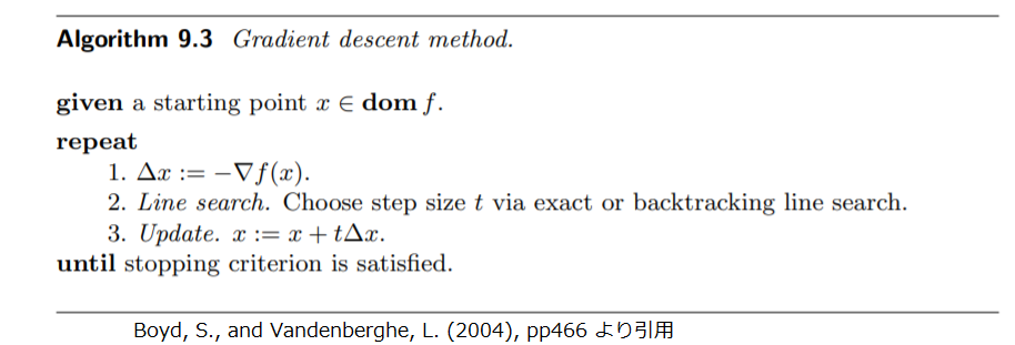
f:id:seetheworld1992:20201119185012p:plain

よく用いられる停止条件は小さい正の整数を {\displaystyle \eta } として {\displaystyle \left\| \nabla f(x) \right\|_2 \le \eta } の形式です.ほどんどの実装において,この条件はステップ1の後に判定されます.


[ 2. 勾配降下法の収束解析 ]

目的関数に強凸性を仮定し,厳密直線探索あるいはバックトラッキング直線探索と組み合わせるときの勾配降下法の収束について調べていきます.


[ 2.1. 勾配降下法と強凸性の仮定による不等式 ]

目的関数 {\displaystyle f(x) }{\displaystyle x \in S } で強凸であると仮定します.すると以下をみたす {\displaystyle m \gt 0, M \gt 0, m \lt M } が存在します.冒頭の過去記事(制約なし凸最適化問題の目的関数)(1.3.1)です.

(2.1.1){\displaystyle \;\;\; m I \preceq \nabla^2 f(x) \preceq M I, \;\;\; x \in S }

以下のステップサイズ {\displaystyle t } の関数 {\displaystyle \tilde{f} : \mathbb{R} \to \mathbb{R} } を定義します.

(2.1.2){\displaystyle \;\;\; \tilde{f}(t) = f(x - t \nabla f(x)), \;\; x - t \nabla f(x) \in S }

強凸性を仮定することにより得られる不等式である冒頭の過去記事(制約なし凸最適化問題の目的関数)(1.2.2)で,{\displaystyle y = x - t \nabla f(x) } として以下を得ます.{\displaystyle \tilde{f}(t) }{\displaystyle t } の二次関数により上から抑えられることを意味します.

(2.1.3){\displaystyle \;\; f(y) \le f(x) + \nabla f(x)^T (y - x) + \frac{M}{2} \left\| y - x \right\|_2^2 }

{\displaystyle \;\;\; \Rightarrow \ f(x - t \nabla f(x)) \le f(x) + \nabla f(x)^T \left( \left(x - t \nabla f(x) \right) - x \right) + \frac{M}{2} \left\| (x - t \nabla f(x)) - x \right\|_2^2 }

{\displaystyle \;\;\;\;\;\;\; \Leftrightarrow \ \tilde{f}(t) \le f(x) + \nabla f(x)^T (- t \nabla f(x)) + \frac{M}{2} \left\| - t \nabla f(x) \right\|_2^2 \;\;\; \because } (2.1.2)

{\displaystyle \;\;\;\;\;\;\;\;\;\;\;\;\;\;\;\;\;\;\;\; = f(x) - t \left\| \nabla f(x) \right\|_2^2 + \frac{M t^2}{2} \left\|  \nabla f(x) \right\|_2^2  \;\;\;\;\;\; } (2.1.3)(※)

{\displaystyle \;\;\;\;\;\;\;\;\;\;\;\;\;\;\;\;\;\;\;\; = f(x) + \left\|  \nabla f(x) \right\|_2^2 \left( \frac{M t^2}{2} - t \right) }

{\displaystyle \;\;\;\;\;\;\;\;\;\;\;\;\;\;\;\;\;\;\;\; = f(x) + \frac{M}{2} \left\|  \nabla f(x) \right\|_2^2 \left( t^2 - \frac{2}{M}  t  \right) }

{\displaystyle \;\;\;\;\;\;\;\;\;\;\;\;\;\;\;\;\;\;\;\; = f(x) + \frac{M}{2} \left\|  \nabla f(x) \right\|_2^2 \left( t - \frac{1}{M} \right)^2 - \frac{M}{2} \left\|  \nabla f(x) \right\|_2^2 \frac{1}{M^2} }

{\displaystyle \;\;\;\;\;\;\;\;\;\;\;\;\;\;\;\;\;\;\;\; = \frac{M}{2} \left\|  \nabla f(x) \right\|_2^2 \left( t - \frac{1}{M} \right)^2 + f(x) - \frac{1}{2M} \left\|  \nabla f(x) \right\|_2^2  \;\;\;\;\;\; } (2.1.3)(※※)


[ 2.2. 厳密直線探索 ]

勾配降下法(1.1.1)を用いるとします.{\displaystyle \tilde{f} } を最小化する {\displaystyle t = t_{\mathrm{exact}} } は以下です.この操作は、厳密直線探索(冒頭の過去記事(降下法の枠組み)(1.2.1)です)を行うことに相当します.

(2.2.1){\displaystyle \;\;\; t_{\mathrm{exact}} = \mathrm{arg \ min}_{ t \ge 0 } \ \tilde{f}(t) }

{\displaystyle \;\;\;\;\;\;\;\;\;\;\;\;\;\;\;\;\;\;\;  = \mathrm{arg \ min}_{ s \ge 0 } \ f( x - s \nabla f(x) ) \;\;\; \because } (2.1.2)

(2.2.2){\displaystyle \;\;\;\tilde{f}(t_{\mathrm{exact}}) = f( x - t_{\mathrm{exact}} \nabla f(x) ) }

以下を定義します.

(2.2.3){\displaystyle \;\;\; c = 1 - m / M \; ( \lt 1 ) }

ここで(2.1.3)(※※)の左辺を {\displaystyle t = t_{\mathrm{exact}} } として最小化し,右辺を {\displaystyle t } の二次関数なので {\displaystyle t = 1/M } として最小化して以下を得ます.

(2.2.4){\displaystyle \;\;\; \tilde{f}(t_{\mathrm{exact}}) \le f(x) - \frac{1}{2M} \left\|  \nabla f(x) \right\|_2^2 }

{\displaystyle \Leftrightarrow \ f( x - t_{\mathrm{exact}} \nabla f(x) ) \le f(x) - \frac{1}{2M} \left\|  \nabla f(x) \right\|_2^2 \;\;\; \because } (2.2.2)

{\displaystyle \;\;\;\;\;\;\;\;\;\; \Leftrightarrow \ f(x^{+}) \le f(x) - \frac{1}{2M} \left\|  \nabla f(x) \right\|_2^2 \;\;\; \because } 冒頭の過去記事(降下法の枠組み)(1.1.2)

{\displaystyle \;\;\;\;\;\; \Leftrightarrow \ f(x^{+}) - p^* \le f(x) - p^* - \frac{1}{2M} \left\|  \nabla f(x) \right\|_2^2  }

{\displaystyle \;\;\;\;\;\;\;\;\;\;\;\;\;\;\;\;\;\;\;\;\;\;\;\;\;\;\;\; \le f(x) - p^* - \frac{1}{2M} 2 m ( f(x) - p^* )  }
{\displaystyle \;\;\;\;\;\;\;\;\;\;\;\;\;\;\;\;\;\;\;\;\;\;\;\;\;\;\;\;\;\;\;\;\;\;\;\;\;\;\;\;\;\;\;\;\;\;\;\;\;\;\;\;\;\;\;\; \because } 冒頭の過去記事(制約なし凸最適化問題の目的関数)(1.1.5)

{\displaystyle \;\;\;\;\;\;\;\;\;\;\;\;\;\;\;\;\;\;\;\;\;\;\;\;\;\;\;\; =  \left( 1 - m / M \right) ( f(x) - p^* ) }

{\displaystyle \;\;\;\;\;\;\;\;\;\;\;\;\;\;\;\;\;\;\;\;\;\;\;\;\;\;\;\; = c ( f(x) - p^* ) \;\;\; \because } (2.2.3)

{\displaystyle \;\;\;\;\; \Leftrightarrow \ f(x^{(k)}) - p^* \le c \ ( f(x^{(k-1)}) - p^* ) \;\;\; \because } 冒頭の過去記事(降下法の枠組み)(1.1.1)(1.1.2)

{\displaystyle \;\;\;\;\;\;\;\;\;\;\;\;\;\;\;\;\;\;\;\;\;\;\;\;\;\;\;\;  \le c^2 ( f(x^{(k-2)}) - p^* ) }
{\displaystyle \;\;\;\;\;\;\;\;\;\;\;\;\;\;\;\;\;\;\;\;\;\;\;\;\;\;\;\;  \cdot \cdot \cdot  }
{\displaystyle \;\;\;\;\;\;\;\;\;\;\;\;\;\;\;\;\;\;\;\;\;\;\;\;\;\;\;\;  \le c^k ( f(x^{(0)}) - p^* ) \;\;\;\;\;\; } (2.2.4)(※)

{\displaystyle \;\;\;\;\;\;\;\;\;\;\;\;\;\;\;\;\;\;\;\;\;\;\;\;\;\;\;\;  \to 0, \;\;\;\;\;\; k \to \infty }

{\displaystyle \;\;\;\;\; \Rightarrow \;\;\; \lim_{k \to \infty} f(x^{(k)}) = p^* }

これより {\displaystyle \epsilon \gt 0 } について以下が成り立ちます.

(2.2.5){\displaystyle \;\;\;   [ c^k ( f(x^{(0)}) - p^* ) \le \epsilon ] \ \Rightarrow \ [ f(x^{(k)}) - p^* \le \epsilon ] }

したがって {\displaystyle f(x^{(k)}) - p^* \le \epsilon }十分条件となる厳密直線探索と勾配降下法の反復回数 {\displaystyle k } の下界は高々以下の回数です.

(2.2.6){\displaystyle \;\;\; c^k ( f(x^{(0)}) - p^* ) \le \epsilon }

{\displaystyle \;\;\;\;\;\;\;\;\; \Leftrightarrow \ c^k \le \epsilon / ( f(x^{(0)}) - p^* ) \;\;\; \because p^* \lt f(x^{(0)}) }

{\displaystyle \;\;\;\;\;\;\;\;\; \Leftrightarrow \ k \log c   \le \log \left[  \epsilon / ( f(x^{(0)}) - p^* ) \right] \;\;\; \because } 両辺とも正

{\displaystyle \;\;\;\;\;\;\;\;\; \Leftrightarrow \ k \ge \frac{ \log \left[  \epsilon / ( f(x^{(0)}) - p^* ) \right] }{ \log c } \;\;\; \because 0 \lt c \lt 1 } より {\displaystyle \log c \lt 0 }

{\displaystyle \;\;\;\;\;\;\;\;\;\;\;\;\;\;\;\;\;  = \frac{ - \log \left[ ( f(x^{(0)}) - p^* ) / \epsilon  \right] }{ - \log (1/c) } }

{\displaystyle \;\;\;\;\;\;\;\;\;\;\;\;\;\;\;\;\;  = \frac{ \log \left[ ( f(x^{(0)}) - p^* ) / \epsilon  \right] }{ \log (1/c) } \;\;\;\;\;\; } (2.2.6)(※)

(2.2.6)(※)の分子 {\displaystyle \log \left[ ( f(x^{(0)}) - p^* ) / \epsilon \right] } は初期の準最適性(すなわち {\displaystyle f(x^{(0)}) }{\displaystyle p^* } のギャップ)の最期の準最適性({\displaystyle \epsilon } より小さい)に対する比の対数をとったものです.この項により,反復回数の下界は,初期点 {\displaystyle x^{(0)} } がどの程度良い点であるか(初期点が良いほど回数が少なくて済む),最終的に必要な精度はどれくらいか(必要な精度が悪いほど回数が少なくて済む),に依存することがわかります.

(2.2.6)(※)の分母 {\displaystyle \log (1/c) } は(2.2.3)より {\displaystyle M/m } の関数です.これは冒頭の過去記事(制約なし凸最適化問題の目的関数)(1.3.13)より行列 {\displaystyle \nabla^2 f(x^*) } の条件数の上界,あるいは同記事(1.3.10)より劣位集合 {\displaystyle \{ z | f(z) \le \alpha \} } の条件数の上界です.その上界 {\displaystyle M/m } が非常に大きいとすると {\displaystyle m/M } は非常に小さく,このとき以下を得ます.

(2.2.7){\displaystyle \;\;\; \log (1/c) = - \log c  }

{\displaystyle \;\;\;\;\;\;\;\;\;\;\;\;\;\;\;\;\;\;\;\;\;\;\;\; = - \log (1 - m/M) \;\;\; \because } (2.2.3)

{\displaystyle \;\;\;\;\;\;\;\;\;\;\;\;\;\;\;\;\;\;\;\;\;\;\;\; \approx m / M  \;\;\;\;\;\; \because \; \log ( 1 +  x ) } の原点まわりのテイラー展開

したがって反復回数 {\displaystyle k } の下界は {\displaystyle M / m } の増加に伴い近似的に線形に増加します.

{\displaystyle \nabla^2 f(x)} の条件数が {\displaystyle x^* } の近くで大きいとき,必要とされる反復回数は大きくなります.逆に,{\displaystyle f(x) } の劣位集合が等方的であり条件数の上界 {\displaystyle M/m } が比較的小さいとき, {\displaystyle c } は小さくなるので(2.2.4)(※)はこのとき収束が速いことを示しています.

(2.2.4)(※)は {\displaystyle f(x^{(k)}) - p^* }等比数列と同じ速さで零に収束することを示しています.数値計算における反復法の文脈において,これを一次収束(linear convergence)といいます.


[ 2.3. バックトラッキング直線探索 ]

勾配降下法とバックトラッキング直線探索を用いるとします.この設定の下,バックトラッキング直線探索の停止条件は以下です(冒頭の過去記事(降下法の枠組み)(1.3.1)にあります).

(2.3.1){\displaystyle \;\;\; f(x + t \Delta x) \le f(x) + \alpha t \nabla f(x)^T \Delta x }

{\displaystyle \;\;\; \Leftrightarrow \ f(x - t \nabla f(x)) = f(x) + \alpha t \nabla f(x)^T ( - \nabla f(x) ) \;\;\; \because } (1.1.1)

{\displaystyle \;\;\;\;\;\;\;\;\;\;\;\;\;\;\;\;\;\;\;\;\;\;\;\;\;\;\;\;\;\; \le f(x) - \alpha t \left\|  \nabla f(x) \right\|_2^2  }

{\displaystyle \;\;\;\;\;\;\;\;\;\;\;\;\;\;\;\;\;\; \Leftrightarrow \ \tilde{f}(t) \le f(x) - \alpha t \left\|  \nabla f(x) \right\|_2^2 \;\;\; \because } (2.1.2)

以下を準備します.

(2.3.2){\displaystyle \;\;\; 0 \le t \le 1/M }

{\displaystyle \;\;\;\;\;\;\;\;\; \Rightarrow \ M t \le 1 \;\;\; \because M \gt 0 }

{\displaystyle \;\;\;\;\;\;\;\;\; \Rightarrow \ M t^2 / 2 \le t/2  }

{\displaystyle \;\;\;\;\;\;\;\;\; \Leftrightarrow \ - t + M t^2 / 2 \le - t/2  }

勾配降下法と目的関数 {\displaystyle f(x) } の強凸性を仮定することにより得られる不等式(2.1.3)より以下を得ます.ただし {\displaystyle t \in [ 0 , 1/M ] } とします.

(2.3.3){\displaystyle \;\;\; \tilde{f}(t) \le f(x) - t \left\| \nabla f(x) \right\|_2^2 + \frac{M t^2}{2} \left\|  \nabla f(x) \right\|_2^2  \;\;\; \because } (2.1.3)(※)

{\displaystyle \;\;\;\;\;\;\;\;\;\;\;\;\;\;\;\;\;\; = f(x) + \left( - t + \frac{M t^2}{2} \right) \left\|  \nabla f(x) \right\|_2^2  }

{\displaystyle \;\;\;\;\;\;\;\;\;\;\;\;\;\;\;\;\;\; \le f(x) + \left( - t / 2 \right) \left\|  \nabla f(x) \right\|_2^2 \;\;\; \because } (2.3.2)

{\displaystyle \;\;\;\;\;\;\;\;\;\;\;\;\;\;\;\;\;\; \le f(x) - \alpha t \left\|  \nabla f(x) \right\|_2^2 }
{\displaystyle \;\;\;\;\;\;\;\;\;\;\;\;\;\;\;\;\;\;\;\;\;\;\;\;\;\;\;\;\;\;\;\;\;\;\;\;\;\;\;\;\;\;\;\;\;\; \because } 冒頭の過去記事(降下法の枠組み)Algorithm 9.2より {\displaystyle \alpha \lt 1/2 }

これはバックトラッキング直線探索の停止条件(2.3.1)と同じものです.したがって {\displaystyle t \in [0,1/M ] } となったときバックトラッキング直線探索は終了します.ここで,バックトラッキング直線探索が {\displaystyle t = t_{N-1} } で終了せず {\displaystyle t = t_{N} } で終了するとします.このとき以下を得ます.

(2.3.4){\displaystyle \;\;\; 1/M \lt t_{N-1} }

{\displaystyle \;\;\;\;\;\;\;\;\; \Leftrightarrow \ \beta / M \lt \beta t_{N-1} \;\;\; \because \beta \in (0,1) }

{\displaystyle \;\;\;\;\;\;\;\;\;\;\;\;\;\;\;\;\;\;\;\;\;\;\; = t_{N} }

{\displaystyle \;\;\;\;\;\;\;\;\; \Rightarrow \ \beta / M \le t_{N}  }

したがってバックトラッキング直線探索は {\displaystyle t = 1 } あるいは {\displaystyle \beta / M \le t } のどちらかのとき終了します.(2.3.3)と冒頭の過去記事(降下法の枠組み)(1.1.2)より以下を得ます.

(2.3.5){\displaystyle \;\;\; f(x^{+}) \le f(x) - \alpha \left\| \nabla f(x) \right\|_2^2 }

(2.3.6){\displaystyle \;\;\; f(x^{+}) \le f(x) - (\beta \alpha / M)  \left\| \nabla f(x) \right\|_2^2 }

併せると以下を得ます.

(2.3.7){\displaystyle \;\;\; f(x^{+}) \le f(x) - \min \{ \alpha , \beta \alpha / M \}  \left\| \nabla f(x) \right\|_2^2 }

{\displaystyle \;\;\; \Leftrightarrow \ f(x^{+}) - p^* \le f(x) - p^* - \min \{ \alpha , \beta \alpha / M \}  \left\| \nabla f(x) \right\|_2^2 }

{\displaystyle \;\;\;\;\;\;\;\;\;\;\;\;\;\;\;\;\;\;\;\;\;\;\;\;\;  \le f(x) - p^* - \min \{ \alpha , \beta \alpha / M \} \left[ 2m(f(x)-p^*) \right] }
{\displaystyle \;\;\;\;\;\;\;\;\;\;\;\;\;\;\;\;\;\;\;\;\;\;\;\;\;\;\;\;\;\;\;\;\;\;\;\;\;\;\;\;\;\;\;\;\;\;\;\;\;\;\;\;\;\;\; \because } 冒頭の過去記事(制約なし凸最適化問題の目的関数)(1.1.5)

{\displaystyle \;\;\;\;\;\;\;\;\;\;\;\;\;\;\;\;\;\;\;\;\;\;\;\;\;  = f(x) - p^* - \min \{ 2 m \alpha , 2 m \beta \alpha / M \} (f(x)-p^*) }

{\displaystyle \;\;\;\;\;\;\;\;\;\;\;\;\;\;\;\;\;\;\;\;\;\;\;\;\;  = (1 - \min \{ 2 m \alpha , 2 \beta \alpha m / M \} )(f(x) - p^*) }

以下を定義します.(2.2.3)と同じ記号ですが許容します.

(2.3.8){\displaystyle \;\;\; c = 1 - \min \{ 2 m \alpha , 2 \beta \alpha m / M \} \; ( \lt 1 ) }

したがって前節の(2.2.4)(※)とほぼ同じ以下を得ます.したがって前節(2.2.5)以下にある収束に関する議論と類似した議論が可能です.

(2.3.9){\displaystyle \;\;\; f(x^{(k)}) - p^* = c^k ( f(x^{(0)}) - p^* )   }

{\displaystyle \;\;\;\;\; \Rightarrow \;\;\; \lim_{k \to \infty} f(x^{(k)}) = p^* }

=================================================================================

以上,制約なし凸最適化問題に対する勾配降下法と目的関数に強凸性を仮定するときの収束解析をまとめました.


参考文献
[1] Boyd, S., and Vandenberghe, L. (2004), Convex Optimization, Cambridge University Press.
[2] Mathematics Stack Exchange https://math.stackexchange.com/questions/3256340/why-does-the-gradient-descent-backtracking-line-search-terminate-when-t-ge-be